
Connecting dice and galaxies
Using the Dirichlet distribution to sample galaxy distances
The context
The Dirichlet distribution has appeared recently in the context of discussing how to propagate redshift uncertainties, especially within the context of redshift inference using so-called galaxy phenotypes (e.g. Sánchez & Bernstein 2019, Sánchez et al. 2020 and Myles et al. 2021). This distribution is used a lot as prior in Bayesian statistics, but its usage in the redshift context (or for galaxy survey science, in general) is still very limited. For that reason, I thought it might be helpful to have some discussion about them, to understand what they are used for. That might be more useful than looking at Wikipedia, which is certainly not very useful (at least to me). This is an attempt at that, starting from the beginning.
The example: throwing dice
We are going to show a very simple example here, unrelated to redshifts at all, but that seemed helpful as it’s a real life case for which we have some more intuition than for redshifts.
Let’s say we are given a die, but we don’t know whether it’s a fair die or not, i.e. we don’t know if the probability for each of the 6 possible outcomes is 1/6 for all. Let’s denote these unknown probabilities for each possible outcome as
\[\mathbf{f} = \{f_i\}, \mathrm{with } \: i \in 1,..,6\]But we have the die, so we can throw it as many times as we want, and then we want to use those observations to make hypothesis about the values of $\mathbf{f}$. So we throw the die a number of times and get counts for each of the 6 possible outcomes
\[\mathbf{N} = \{N_i\}, \mathrm{with } \: i \in 1,..,6\]We know the likelihood of observing such counts given a set of intrinsic probabilities for each outcome, \(p(\mathbf{N} \vert \mathbf{f})\), is a multinomial distribution. But we don’t want that, we want the posterior on those probabilities, given that we have observed those counts. For that posterior, we ask Thomas Bayes (or Price or Laplace or whoever), and they tell us that is given by:
\[p(\mathbf{f}|\mathbf{N}) \propto p(\mathbf{N}|\mathbf{f}) p(\mathbf{f})\]The first term on the right is the likelihood, which we said it’s a multinomial. And here is where the Dirichlet enters. The Dirichlet is the conjugate prior of the multinomial distribution. This means that, if we have a multinomial likelihood, and we choose a Dirichlet prior, then the posterior is also Dirichlet distributed.
The Dirichlet distribution is parameterized by a vector of positive reals, ${\boldsymbol{\alpha}}$. In detail, it takes the follwing form:
\[\mathrm{Dir}(\mathbf{f};\boldsymbol{\alpha}) \propto \prod_i f_i^{\alpha_i-1}\]There are some properties we like about the Dirichlet sampling: it gives us samples of probabilities, so they have the right properties of probabilities (all elements positive and adding to one). Also, when all ${\boldsymbol{\alpha}}=1$, that Dirichlet distribution is uniform over the allowed values that probabilities can take. So we can see why this distribution tends to be a resonable choice of prior.
In the case depicted above, the posterior, if we choose a dirichlet prior with a given set of parameters ${\boldsymbol{\alpha}}$, can be written simply as:
\[p(\mathbf{f}|\mathbf{N}) \propto p(\mathbf{N}|\mathbf{f}) p(\mathbf{f}) = \mathrm{Dir}(\mathbf{f};\mathbf{N}+\boldsymbol{\alpha})\]So we are simply summing counts in the likelihood (our evidence) with counts in our prior. There is one other important advantage about using a Dirichlet prior (and hence having a Dirichlet posterior): It makes the posterior very easy to sample from: numpy does it for you (even deprecated numpy!). Let’s try that die case with some simple code.
Importing modules
import numpy as np
import matplotlib.pyplot as plt
%matplotlib inline
plt.rcParams['font.size'] = 16
plt.rcParams['axes.labelsize'] = 16
plt.rcParams['axes.labelweight'] = 'bold'
plt.rcParams['figure.figsize'] = (16.,8.)
import config
import pylab as mplot
%pylab inline
rgb = np.array([(28, 46, 242), (97, 137, 228), (237, 177, 104), (176,56,19)])/255.
colors2 =['midnightblue', rgb[0], rgb[1], rgb[2], rgb[3], 'maroon']
mplot.rc('font', weight='bold')
Populating the interactive namespace from numpy and matplotlib
Possible outcomes for a die
outcomes = np.arange(1,7,1)
print outcomes
[1 2 3 4 5 6]
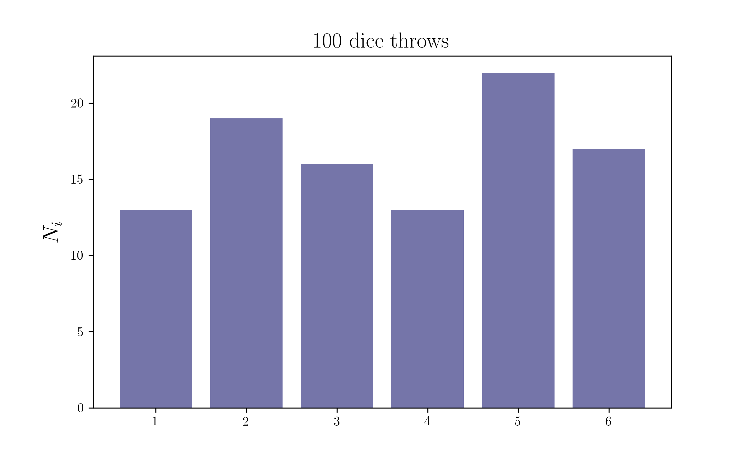
Let’s throw the die 100 times and count them
We will be generating the data with a fair die, with equal probabilities (1/6) for every possible outcome. Hence we expect our posteriors to be compatible with that. You can easily change the probabilities of the die and make it a weighted die by changing the random multinomial draws, and you should recover your input too!
dice_counts = np.random.multinomial(100, [1/6.]*6)
print dice_counts
[15 17 15 21 13 19]
plt.figure(figsize=(8,5))
plt.bar(outcomes,dice_counts,color=colors2[0],alpha=0.6)
plt.title('100 dice throws',size=17)
plt.ylabel(r'$N_i$',size=17)
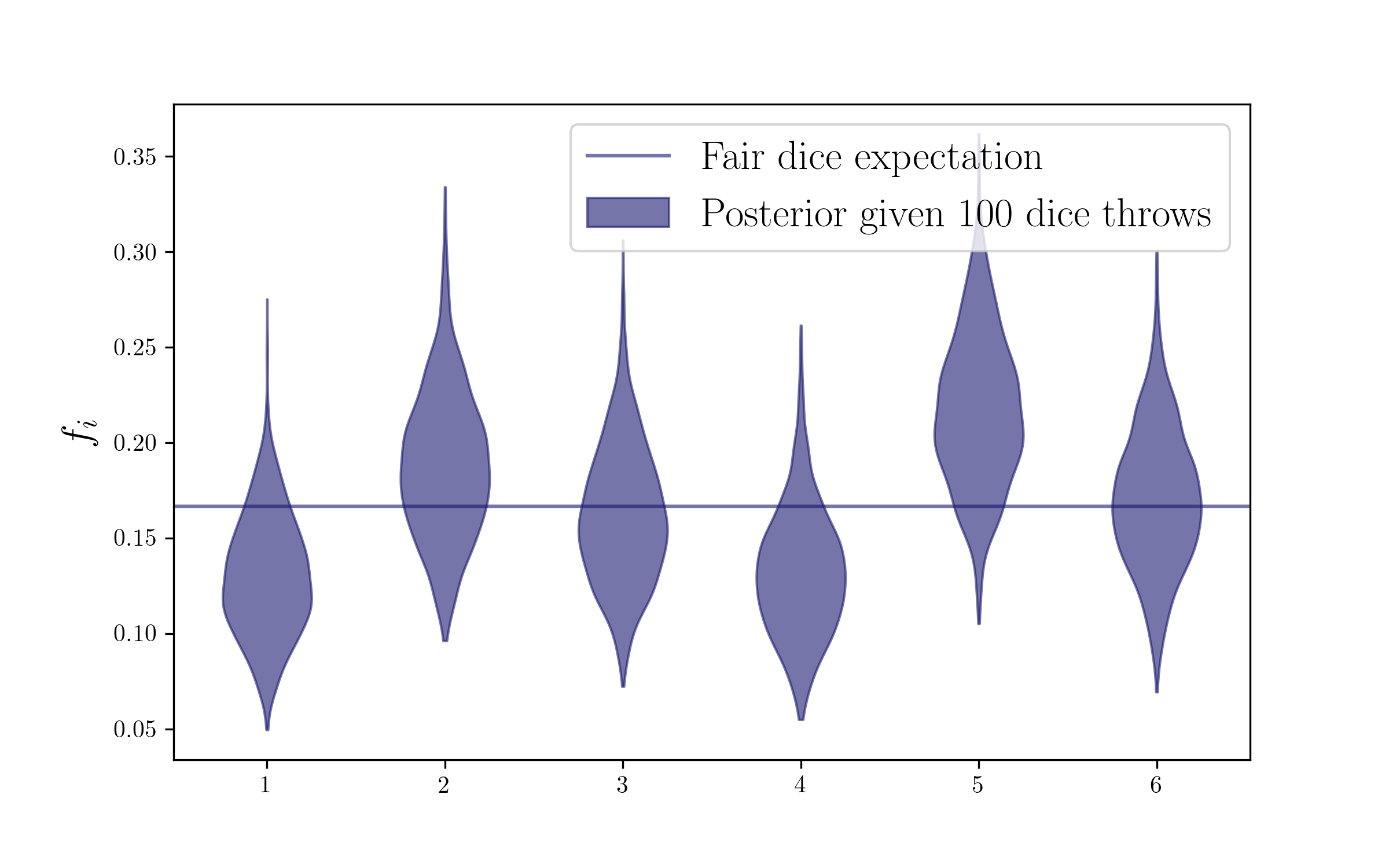
Let’s sample the posterior
Now we have the counts, so we are ready to get the posterior on the probabilities by taking Dirichlet draws on those counts. We are going to add 1 to those counts (meaning that we will use a uniform Dirichlet prior) but you can also check with other choices of the prior counts (adding 1/2 is the Jeffrey prior, or you can try and set a very small number).
ndraws = 1000 # This number of Dirichlet draws for sampling your posterior is arbitrary, you can choose more, for it's very fast!

fs = np.zeros((ndraws,len(outcomes)))
for i in range(ndraws):
    fs[i] = np.random.dirichlet(dice_counts+1)
Plot the posterior
Now we are ready to plot our posterior on the probabilities. We are doing a violin plot, but a corner plot would get the possible correlations too.
plt.figure(figsize=(8,5))
parts = plt.violinplot(
        fs,positions=outcomes, widths=0.5, showmeans=False, showmedians=False, showextrema=False)
for pc in parts['bodies']:
    pc.set_alpha(0.6)
    pc.set_facecolor(colors2[0])
    pc.set_edgecolor(colors2[0])


pc.set_label(r'Posterior given 100 dice throws')

plt.axhline(1/float(len(outcomes)),label='Fair dice expectation',c=colors2[0],alpha=0.6)
plt.legend(fontsize=17)
plt.ylabel(r'$f_i$',size=17)
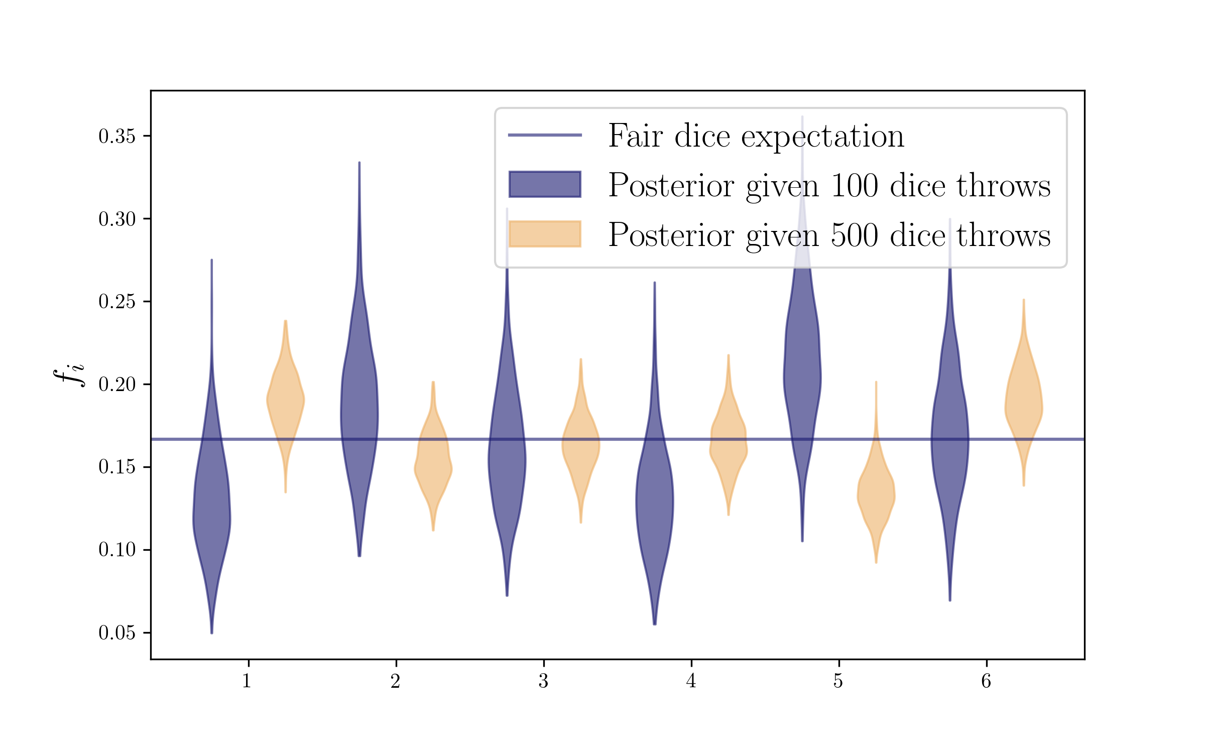
More throws
Now let’s throw the die 500 times. We will have more counts (more evidence, more data), and hence our posterior should shrink!
dice_counts2 = np.random.multinomial(500, [1/6.]*6)
print dice_counts2
[71 84 85 94 87 79]
fs2 = np.zeros((ndraws,len(outcomes)))
for i in range(ndraws):
    fs2[i] = np.random.dirichlet(dice_counts2+1)
plt.figure(figsize=(8,5))
parts = plt.violinplot(
        fs,positions=outcomes-0.25, widths=0.25, showmeans=False, showmedians=False, showextrema=False)
for pc in parts['bodies']:
    pc.set_alpha(0.6)
    pc.set_facecolor(colors2[0])
    pc.set_edgecolor(colors2[0])

pc.set_label(r'Posterior given 100 dice throws')

parts = plt.violinplot(
        fs2,positions=outcomes+0.25, widths=0.25, showmeans=False, showmedians=False, showextrema=False)
for pc in parts['bodies']:
    pc.set_alpha(0.6)
    pc.set_facecolor(colors2[3])
    pc.set_edgecolor(colors2[3])


pc.set_label(r'Posterior given 500 dice throws')


plt.axhline(1/float(len(outcomes)),label='Fair dice expectation',c=colors2[0],alpha=0.6)
plt.legend(fontsize=17)
plt.ylabel(r'$f_i$',size=17)
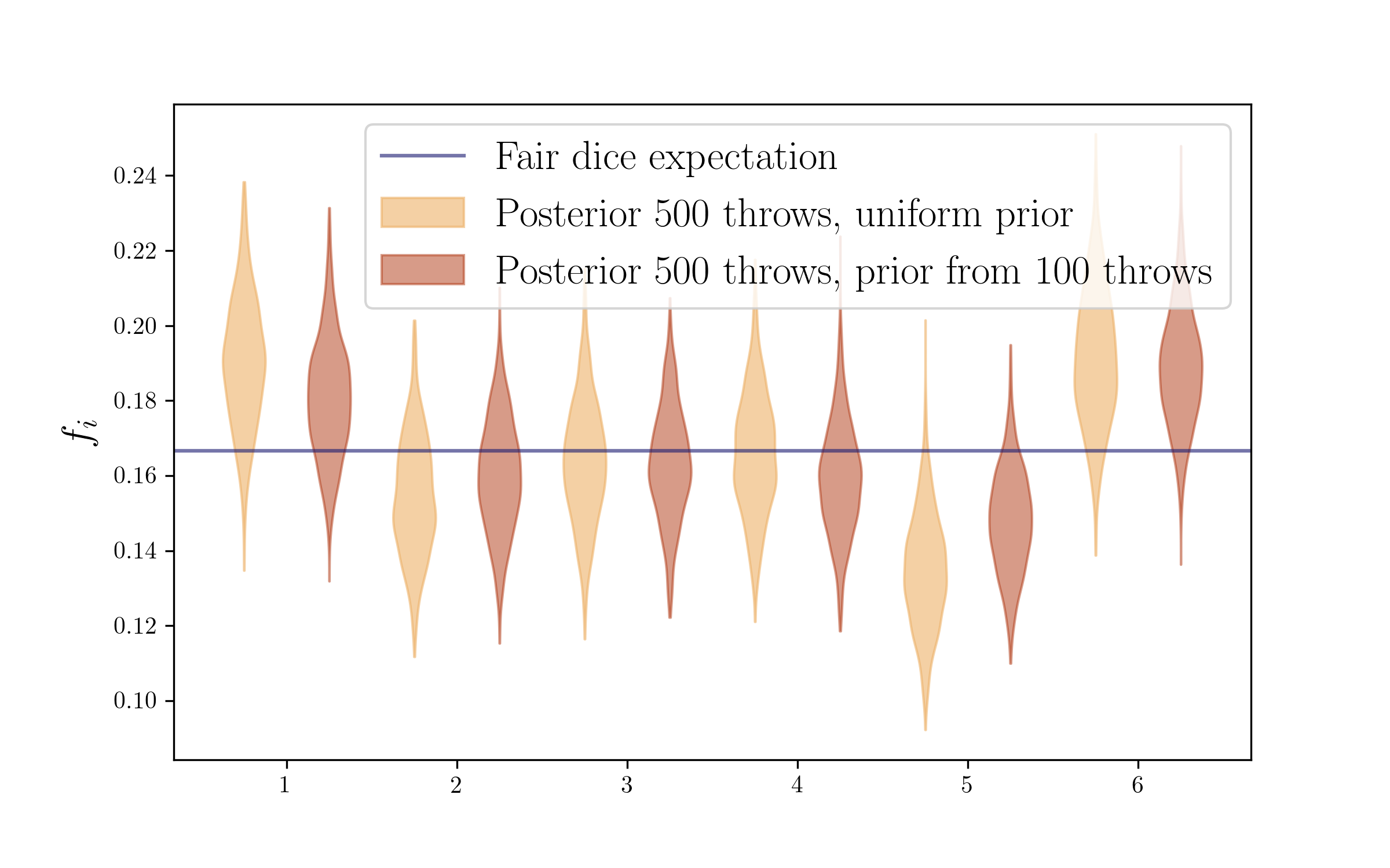
Updating your prior
There is one subtlety here to be considered. We said we had thrown the die a 500 times more, but in getting that posterior, we again used a uniform prior (that +1 adding to the counts). In fact, we already had some information on those probabilities, given by our 100 throws before, so we could have perfectly used those counts as a prior for the new 500 throws. And for doing that we would just add the new and old counts in the Dirichlet draws, as simple as that!
This will make use of all the information. And I think it makes a very intuitive and clear picture of how, from a Bayesian perspective, new evidence does not completely determine your beliefs, it updates your prior beliefs.
fs3 = np.zeros((ndraws,len(outcomes)))
for i in range(ndraws):
    fs3[i] = np.random.dirichlet(dice_counts2+dice_counts)
plt.figure(figsize=(8,5))
parts = plt.violinplot(
        fs2,positions=outcomes-0.25, widths=0.25, showmeans=False, showmedians=False, showextrema=False)
for pc in parts['bodies']:
    pc.set_alpha(0.6)
    pc.set_facecolor(colors2[3])
    pc.set_edgecolor(colors2[3])
pc.set_label(r'Posterior 500 throws, uniform prior')

parts = plt.violinplot(
        fs3,positions=outcomes+0.25, widths=0.25, showmeans=False, showmedians=False, showextrema=False)
for pc in parts['bodies']:
    pc.set_alpha(0.5)
    pc.set_facecolor(colors2[4])
    pc.set_edgecolor(colors2[4])


pc.set_label(r'Posterior 500 throws, prior from 100 throws')

plt.axhline(1/float(len(outcomes)),label='Fair dice expectation',c=colors2[0],alpha=0.6)
plt.legend(fontsize=17)
plt.ylabel(r'$f_i$',size=17)
Introducing the issue of correlation
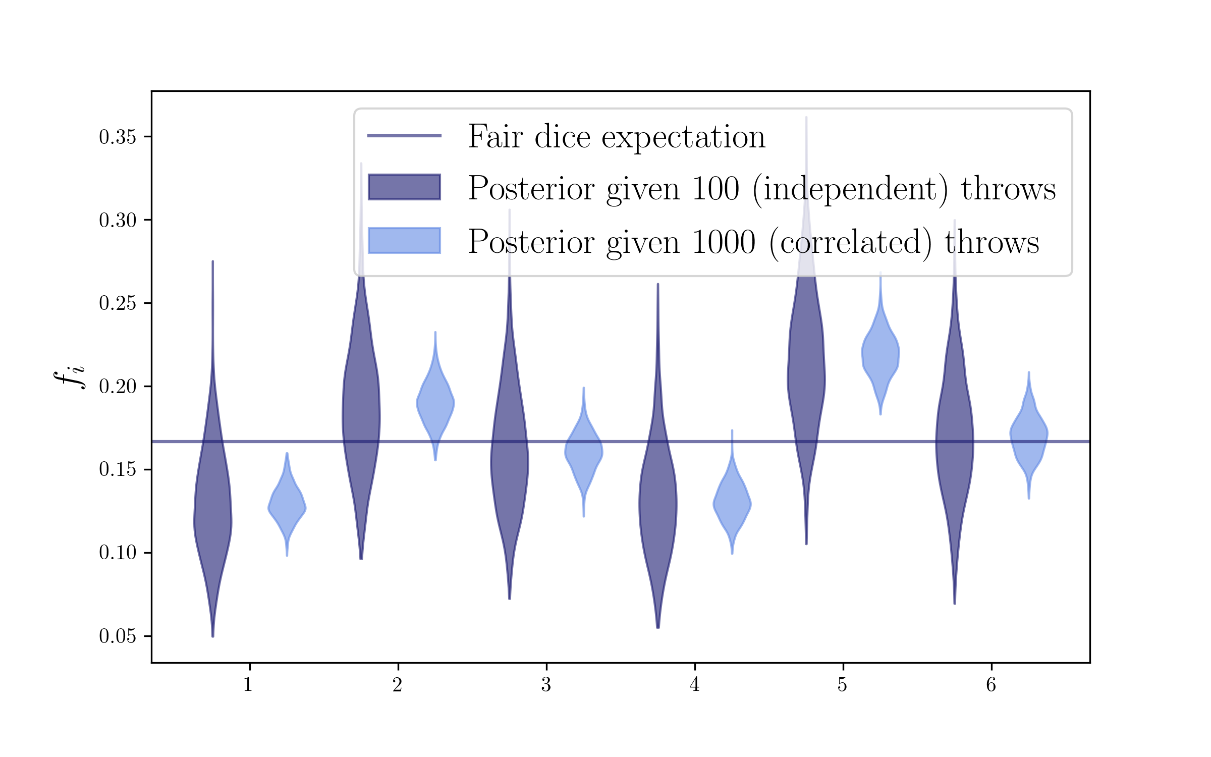
From all these examples above we have seen that having more counts (more data) will shrink the posterior distribution we sample using the Dirichlet dirstribution. So far we have assumed all our dice throws were independent. However, let’s now imagine the situation in which, for some reason maybe related to bookkeeping, we are double-counting our throws, and hence some of our counts will be correlated. In that case, we will have more counts that actual independent information and hence our posterior may be artificially too tight, and may hence lead us to biases in our posterior beliefs. Let’s look at a rather extreme example, where we are counting each of our 100 throws 10 times, so we will have 1000 throws but only 100 of them will be independent.
dice_counts_corr = dice_counts*10
print dice_counts_corr
[150 170 150 210 130 190]
fs_corr = np.zeros((ndraws,len(outcomes)))
for i in range(ndraws):
    fs_corr[i] = np.random.dirichlet(dice_counts_corr+1)
plt.figure(figsize=(8,5))
parts = plt.violinplot(
        fs,positions=outcomes-0.25, widths=0.25, showmeans=False, showmedians=False, showextrema=False)
for pc in parts['bodies']:
    pc.set_alpha(0.6)
    pc.set_facecolor(colors2[0])
    pc.set_edgecolor(colors2[0])


pc.set_label(r'Posterior given 100 (independent) throws')

parts = plt.violinplot(
        fs_corr,positions=outcomes+0.25, widths=0.25, showmeans=False, showmedians=False, showextrema=False)
for pc in parts['bodies']:
    pc.set_alpha(0.6)
    pc.set_facecolor(colors2[2])
    pc.set_edgecolor(colors2[2])


pc.set_label(r'Posterior given 1000 (correlated) throws')

plt.axhline(1/float(len(outcomes)),label='Fair dice expectation',c=colors2[0],alpha=0.6)
plt.legend(fontsize=17)
plt.ylabel(r'$f_i$',size=17)
Scaling the counts in the Dir
From the last plot, we can see that having correlated data in our Dirichlet posterior can lead to underestimating our posterior uncertainties and hence lead to biased posterior beliefs. How can we correct for this?
Well, one way around this can be to scale down our counts in the Dirichlet to account for the average correlation in the input counts, i.e.
\[\mathrm{Dir}(\mathbf{f};\mathbf{N}) \rightarrow \mathrm{Dir}(\mathbf{f};\mathbf{N/\lambda})\]where $\lambda$ is an estimate of the average correlation in the sample (in the example above would be 10 to bring back the posterior uncertainties to the right answer). Note that when using a constant scaling of the counts in the Dirichlet like this, the expected value of the posterior would not change, but the uncertainties (the width) of the posterior will. In a similar way, having a non-constant scaling in the Dirichlet would not only change our uncertainties but also bias the expected value of the posterior, so we don’t want to do that. Finally, please also note that upscaling counts (i.e. having a lambda smaller than 1) will be dangerous, as you will be assuming you have more information than you do, and you’ll probably end up underestimating your uncertainties and hence biasing your posterior.
Connection to redshifts
Now let’s try to connect some of this to the redshift case. We can imagine that our dice experiment corresponds to the redshift probabilities of something (maybe a Self-Orginizing Map cell using deep photometry, as in Sánchez et al. 2020), so that redshift can take one of each of these 6 values. We have some observations that give us counts for each of the 6 redshift bins, and we use the Dirichlet draws to sample the redshift posterior distribution of those 6 bins based on the observations, and some Dirichlet prior of your choice.
And now let’s connect to the sample variance issue as well. The example of double-counting your die can be similar to the effect of sample variance in the redshift case. If your redshift counts come from an observation of a small area in a given line of sight (LOS), then you will have structures along that LOS. If you encounter a galaxy cluster at a given redshift, you are likely to be finding a lot more redshift counts at that specific redshift of the galaxy cluster than you would otherwise do for larger area, not so much dominated by sample variance (with more clusters and voids to average out). So sample variance is effectively making us double-count our redshifts, i.e. introducing correlations in the counts we want to input our Dirichlet sampling. This is the reason for us to use a scaling
\[\mathrm{Dir}(\mathbf{f};\mathbf{N}) \rightarrow \mathrm{Dir}(\mathbf{f};\mathbf{N/\lambda})\]to correct for that correlation, as long as we can estimate the average correlation introduced by sample variance. This is the main idea behind our Dirichlet application to the sample variance problem, described in detail in this paper.
There is one (or two) complications when applying this idea to the redshift sample variance problem though, which are the reason for that complicated 3-step Dirichlet sampling. One is that we need a constant scaling not to bias our posterior, but sample variance itself depends on redshift (it is more important at low redshift, where we probe a smaller volume). That is, for sample variance, we want to inflate the uncertainty of the redshift distribution posterior, but we want that uncertainty to depend on redshift. And this is the reason we need to do more than one step in the Dirichlet sampling, also sampling over phenotypes. Then there is an additional problem, which is that phenotypes correlate heavily with each other in redshift, and hence we group them together by redshift proximity, to make them independent, and that is the reason for the additional third step.
This whole sampling process is explained in more detail in the paper, but hopefully the correlated dice analogy, and how to correct for it scaling down the input counts in the Dirichlet, gives us some intuition about the main idea behind it. And it is fun to connect dice and galaxies!
This tutorial was presented and shared within the Redshift Working Group of the Dark Energy Suvey collaboration, and also within the cosmology groups at the University of Pennsylvania and Carnegie Mellon University, some time during the summer of 2020.