
Writing a simple Monte Carlo Markov Chain code
And apply it to a simple, real data example
Introduction and Bayes theorem
Before we go into the fun part, let’s start with some short (and probably incomplete) introduction. We will be working here in the context of parameter inference, i.e., we want to know the probability of our model parameters given the data. In particular, we are interested in estimating the posterior probability distribution function of each parameter \(\theta\) in our model \(M\) given the data \(D\), \(p(\theta |M,D)\). Bayes theorem relates that posterior distribution to the likelihood, \(\mathcal{L}(D|\theta,M)\), computed from the model and the data, and the prior, \(\pi(\theta|M)\), which encapsulates a priori information we may have on the parameters of our model, via the following equation:
\[p(\theta |M,D) = \frac{\mathcal{L}(D|\theta,M) \pi(\theta|M)}{p(D|M)}\]where the denominator on the right is called the evidence, which will just be a normalizing constant for us, since it is not required for parameter inference given a model but it is essential in problems of model selection, when comparing two or more different models to see which of them is favored by the data. In summary, we want to get the posterior of the parameters, and we will do it by using the likelihood and the prior.
Procedure and sampling
It will take us a few steps to compute the posterior of our model parameters, namely
- For a given point in parameter space, generate a model prediction
- Compute a probability (likelihood) of the data given that model
- Given some prior, use Bayes theorem to get the posterior at that point in parameter space
- Go to another point in parameter space in order to sample it
The last step on the previous list is a very important one, and actually the main connection between parameter inference and Markov Chain Monte Carlo’s. If we have some model as a function of 2 parameters (say \(\sigma_8,\Omega_m\)), we may be able to go over steps 1-3 in our list above for every point in a 2D grid, and get something like this in a reasonable amount of time:
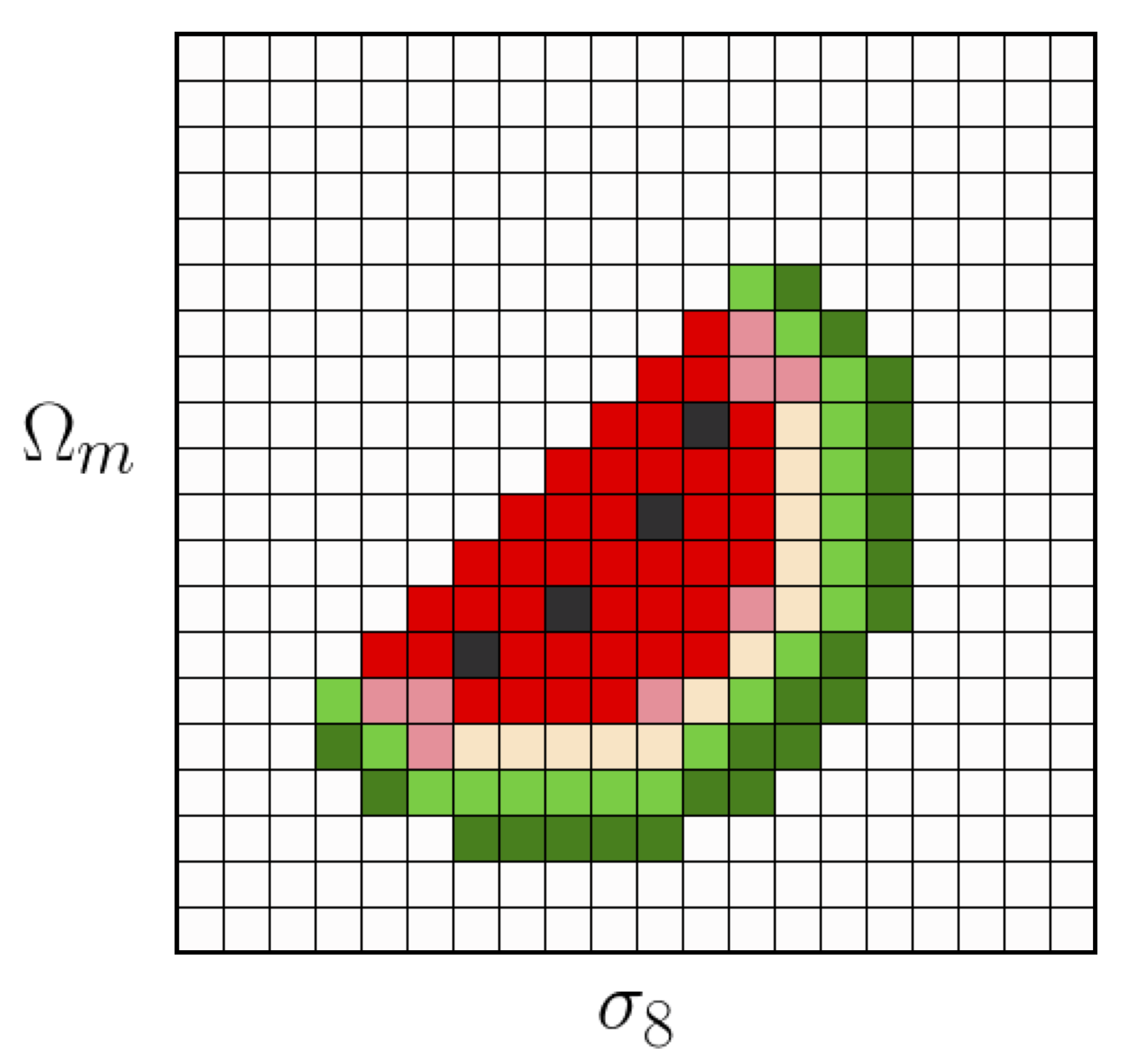
However, nowadays typical cosmological analysis require many more parameters. For instance, the DES Y1 analysis used 6 cosmological parameters for the \(\Lambda CDM\) model (and many more nuisance parameters!). With 6 dimensions, even in a simplified case where our grid only has 20 pixels per dimension, if it takes about 1.5 seconds for each 1-3 evaluation we would need more than 1000 days to sample the whole space!
MCMC’s
MCMCs are much faster at sampling the parameter space than just going over the whole grid. In a few words, MCMCs start at an arbitrary point in parameter space, and then they take Markov steps (memoryless, every new state depends on the current state, and only on the current state), and they sample the parameter space in a way such that density of points is proportional to the posterior probability. They can be thought as a random walk in parameter space, and they are very fast compared to the grid example, and faster than the grid the more dimensions we add to the problem.
Even though there are several different MCMC implementations, here we will focus on the classic Metropolis-Hastings algorithm. The Metropolis algorithm has been placed among the 10 algorithms that have had the greatest influence on the development and practice of science & engineering in the 20th century (Beichl & Sullivan 2000). The algorithm can be described as follows:
Let \(\theta^i\) be the set of parameters of model \(M\) in a given point i in parameter space, and \((\mathcal{L}\pi)^i\) be the product of the likelihood times the posterior at that point, which we will use to estimate the posterior (modulo the normalization) given Bayes theorem. Then, we will take the next steps:
- \(a\)) Start at a random location in parameter space: \(\theta^{old}\), \((\mathcal{L}\pi)^{old}\)
- \(b\)) Try to take a random step in parameter space: \(\theta^{new}\), \((\mathcal{L}\pi)^{new}\)
- \(c_a\)) If \((\mathcal{L}\pi)^{new}\) \(\geq\) \((\mathcal{L}\pi)^{old}\), then accept (take and save) the step, \(new\) \(\rightarrow\) \(old\) and go to step \(b\))
- \(c_b\)) If \((\mathcal{L}\pi)^{new}\) \(<\) \((\mathcal{L}\pi)^{old}\), then draw a random number \(r\) uniform in (0,1)
- If \(r \geq (\mathcal{L}\pi)^{new}/(\mathcal{L}\pi)^{old}\) then do not take the step (i.e. save \(old\)) and go to step \(b\))
- If \(r < (\mathcal{L}\pi)^{new}/(\mathcal{L}\pi)^{old}\) then do as in step \(c_a\))
And keep going like that… The probability distribution of the random step (the step size) is called the proposal distribution, which should not be changed once the chain has started. This distribution is crucial to the MCMC efficiency, in the sense that too small steps will imply poor mixing, and too big steps will result in a poor acceptance rate.
Even if the MCMC will eventually converge to the target distribution, the initial steps in the chain may follow a different distribution, because the starting point may be in a region of low probability. Then, one typically has to throw away a number of steps at the beginning of the chain. This initial part of the chain, useless for parameter estimation, is known as burn in.
The real data
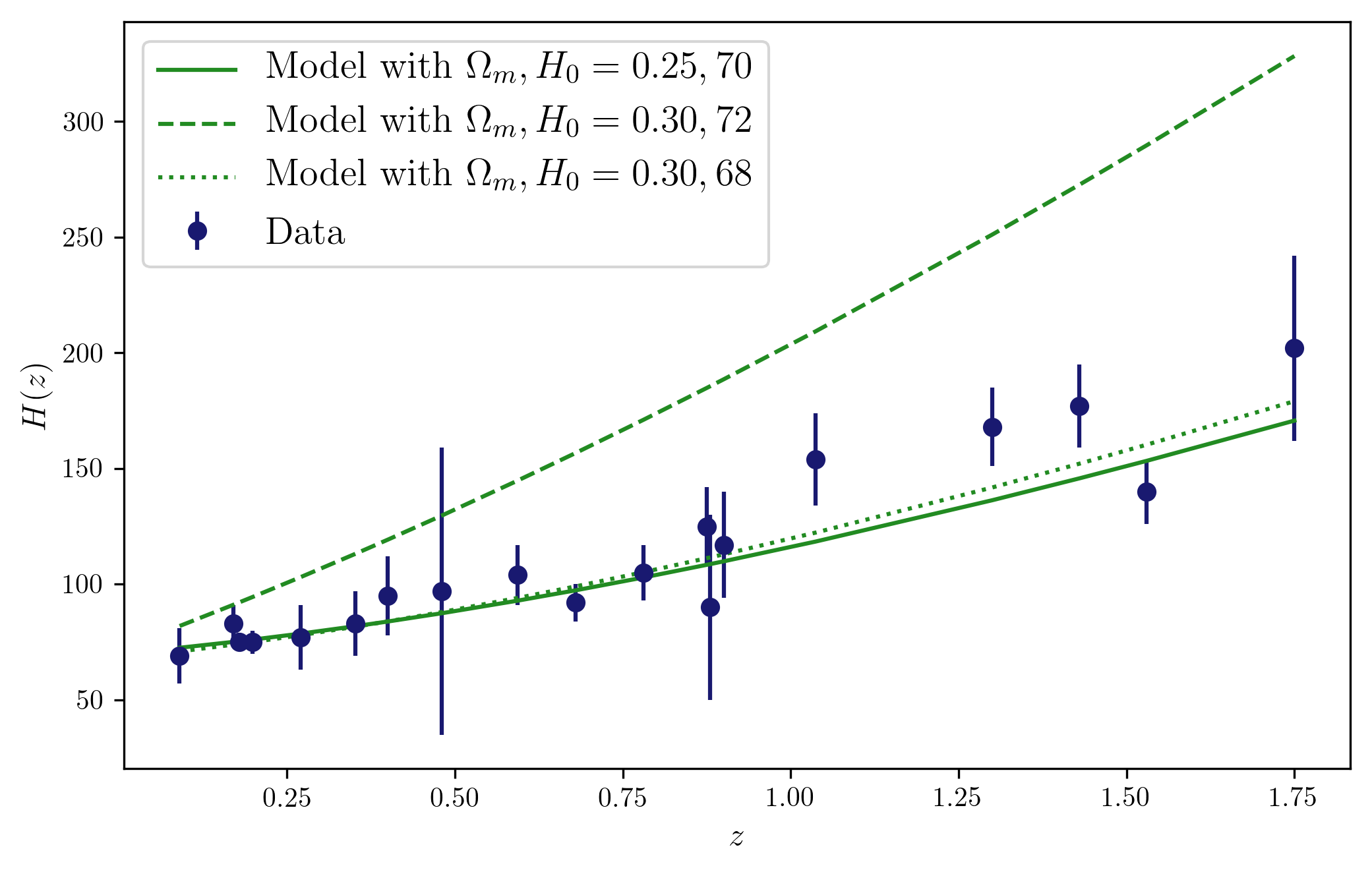
We are gonna be using real data in this exercise. Specifically, from this paper, where they provide a measurement of the expansion history obtained from the ages of passively-evolving galaxies in galaxy clusters at various redshifts. And we’re gonna use the data, \(H(z)\), to constrain the parameters \(H_0\) and \(\Omega_m\) using the model:
\[H(z) = H_0 \sqrt{\Omega_m(1+z)^3+(1-\Omega_m)}\]Now let’s load the data and define the model.
%matplotlib inline
import numpy as np
import numpy.random as rn
import matplotlib.pyplot as plt
#Latex stuff
plt.rc('text', usetex=True)
plt.rc('font', family='serif')
from scipy.stats import gaussian_kde
import scipy.ndimage as ndimage
from matplotlib.ticker import NullFormatter
#Loading the data
z, h, h_err = np.loadtxt('Hz_BC03_all.dat',unpack=True)
#Defining the model as a function of the parameters
def hofz(z,h0,omega_m):
        hofz = h0*np.sqrt(omega_m*(1+z)**3+(1-omega_m))
        return hofz
At this point, we can already look at the data and their comparison to the model given some parameters that we can just choose (so we can see that some paramters will not be a good fit to the data).
plt.figure(figsize=(8,5))
plt.xlabel(r'$z$',size='large')
plt.ylabel(r'$H(z)$',size='large')
plt.errorbar(z,h,h_err,c='midnightblue',ls='',fmt='o',label='Data')
plt.plot(z,hofz(z,70,0.25),c='forestgreen',label=r'Model with $\Omega_m,H_0 = 0.25,70$')
plt.plot(z,hofz(z,72,1),c='forestgreen',ls='dashed',label=r'Model with $\Omega_m,H_0 = 0.30,72$')
plt.plot(z,hofz(z,68,0.3),c='forestgreen',ls='dotted',label=r'Model with $\Omega_m,H_0 = 0.30,68$')
plt.legend(fancybox=True,fontsize=14,loc=2)
Now we can already start writing down the MCMC for these data and model, following the steps above. We can use a Gaussian likelihood and assume the data points are independent. We could also use priors on the parameters, from other experiments for instance, or just use uninformative priors.
Running the chains
The code provided here is just a very simple implementation of the steps described above, and its main purpose is to help us understand what the MCMC is actually doing. However, the code is not optimized, so when using MCMCs in research we will likely use other, more optimal implementations. But trying to code it for yourself is useful to understand the algorithm!
#Defining the likelihood and the (flat) prior
def lik(z,h,herr,h0,omega_m):
        chisq = 0.
        for i in range(len(z)):
                chisq += (h[i] - hofz(z[i],h0,omega_m))**2/(herr[i]**2)
        return np.exp(-chisq/2.)

def prior(h0,omega_m):
    if 50 < h0 < 100 and 0. < omega_m < 1.:
        return 1.0
    return 0.0

# Defining the MCMC, depending on the chain lenght, and the size of the steps on each parameter
def mcmc(nit = 50000, h_step = 1, omega_m_step = 0.025):
    # Defining an array to save 3 numbers at each iteration: h, omega_m and likelihood
    array = np.zeros((nit,3))
    # Start the chain, randomly choosing a point in parameter space
    h_ini, omega_m_ini = rn.uniform(50,100,1), rn.uniform(0.,1.,1)
    like_ini = lik(z,h,h_err,h_ini,omega_m_ini)
    array[0] = h_ini, omega_m_ini, like_ini
    h_old, omega_m_old, like_old = h_ini, omega_m_ini, like_ini
    for i in range(1,nit):
        # Here we define the steps in each parameter, following Gaussian distributions
        dh_i, domega_m_i = rn.normal(0,h_step,1), rn.normal(0,omega_m_step,1)
        h_i, omega_m_i = (h_old+dh_i), (omega_m_old+domega_m_i)
        like = lik(z,h,h_err,h_i,omega_m_i)*prior(h_i,omega_m_i)
        rand = rn.random(1)
        if ((i > 0) & (like >= like_old)):
                array[i] = h_i, omega_m_i, like
                h_old, omega_m_old, like_old = array[i]
        elif ((i > 0) & (like < like_old)):
                if rand >= like/like_old:
                        array[i] = array[i-1]
                if rand < like/like_old:
                        array[i] = h_i, omega_m_i, like
                        h_old, omega_m_old, like_old = array[i]
        else:
                array[i] = array[i-1]
    return array

# Some plots to look at the chains here
def plot_params(array):
    fig, ax = plt.subplots(3,1,sharex=True,figsize=(8,6))
    ax[0].plot(range(len(array[:,1])),array[:,2],c='midnightblue')
    ax[0].set_xscale('log')
    ax[0].set_yscale('log')
    ax[0].set_ylabel(r'Likelihood',size='large')
    ax[1].plot(range(len(array[:,1])),array[:,0],c='midnightblue')
    ax[1].set_ylabel(r'$H_0$',size='large')
    ax[2].plot(range(len(array[:,1])),array[:,1],c='midnightblue')
    ax[2].set_ylabel(r'$\Omega_m$',size='large')
    ax[2].set_xlabel('Step number',size='large')

def plot_chain(array,kde=False):
    # Scatter plot of the chain two parameters
    x = array[:,1]
    y = array[:,0]
    if kde<1:
        plt.figure(figsize=(6,5))
        plt.scatter(x, y, c='midnightblue', s=50, edgecolor='')
        plt.xlabel(r'$\Omega_m$',size='large')
        plt.ylabel(r'$H_0$',size='large')
    else:
        # Using KDE to calculate the density at each point
        xy = np.vstack([x,y])
        zkde = gaussian_kde(xy)(xy)

        # Sort the points by density, so that the densest points are plotted last
        idx = zkde.argsort()
        x, y, zkde = x[idx], y[idx], zkde[idx]
        plt.figure(figsize=(6,5))
        plt.scatter(x, y, c=zkde, s=50, edgecolor='',cmap='viridis')
        plt.xlabel(r'$\Omega_m$',size='large')
        plt.ylabel(r'$H_0$',size='large')
Chain convergence
We will typically run a number of chains starting at different locations in parameter space. Given \(M\) chains with \(N\) elements each, we can compute the so-called Gelmans and Rubin convergence metric for a given parameter, \(y\). The metric is defined from the following quantities:
- The chain mean, \(\bar{y}^j = \frac{1}{N} \sum_{i=1}^N y_i^j\)
- The mean of the distribution, \(\bar{y} = \frac{1}{NM}\sum_{ij=1}^{NM} y_i^j\)
- The variance between chains, \(B = \frac{1}{M-1}\sum_{j=1}^M (\bar{y}^j-\bar{y})^2\)
- And the variance within the chains, \(W = \frac{1}{M(N-1)}\sum_{ij} (y_i^j-\bar{y}^j)^2.\)
From these definitions, the convergence metric reads \(R = \frac{\frac{N-1}{N}W + B(1+\frac{1}{M})}{W},\)
and we should require \(R<1.03\) for ensuring convergence (\(R>1\) by construction).
nsteps = 200000
h0_step = 1
om_step = 0.025
chain1 = mcmc(nsteps,h0_step,om_step)
chain2 = mcmc(nsteps,h0_step,om_step)
chain3 = mcmc(nsteps,h0_step,om_step)
chain4 = mcmc(nsteps,h0_step,om_step)
p = 2 #Parameter: 0:H_0, 1:Omega_m

y1 = np.mean(chain1,axis=0)[p]
y2 = np.mean(chain2,axis=0)[p]
y3 = np.mean(chain3,axis=0)[p]
y4 = np.mean(chain4,axis=0)[p]
v1 = np.var(chain1,axis=0)[p]
v2 = np.var(chain2,axis=0)[p]
v3 = np.var(chain3,axis=0)[p]
v4 = np.var(chain3,axis=0)[p]

N = float(nsteps)
M = 4.
y = np.array([y1,y2,y3,y4])
v = np.array([v1,v2,v3,v4])
B = 1./(M-1)*((y-y.mean())*(y-y.mean())).sum()
W = 1./M*v.sum()
R = ((N-1)/N*W + B*(1+1/M))/W
print R
1.0002795940637148
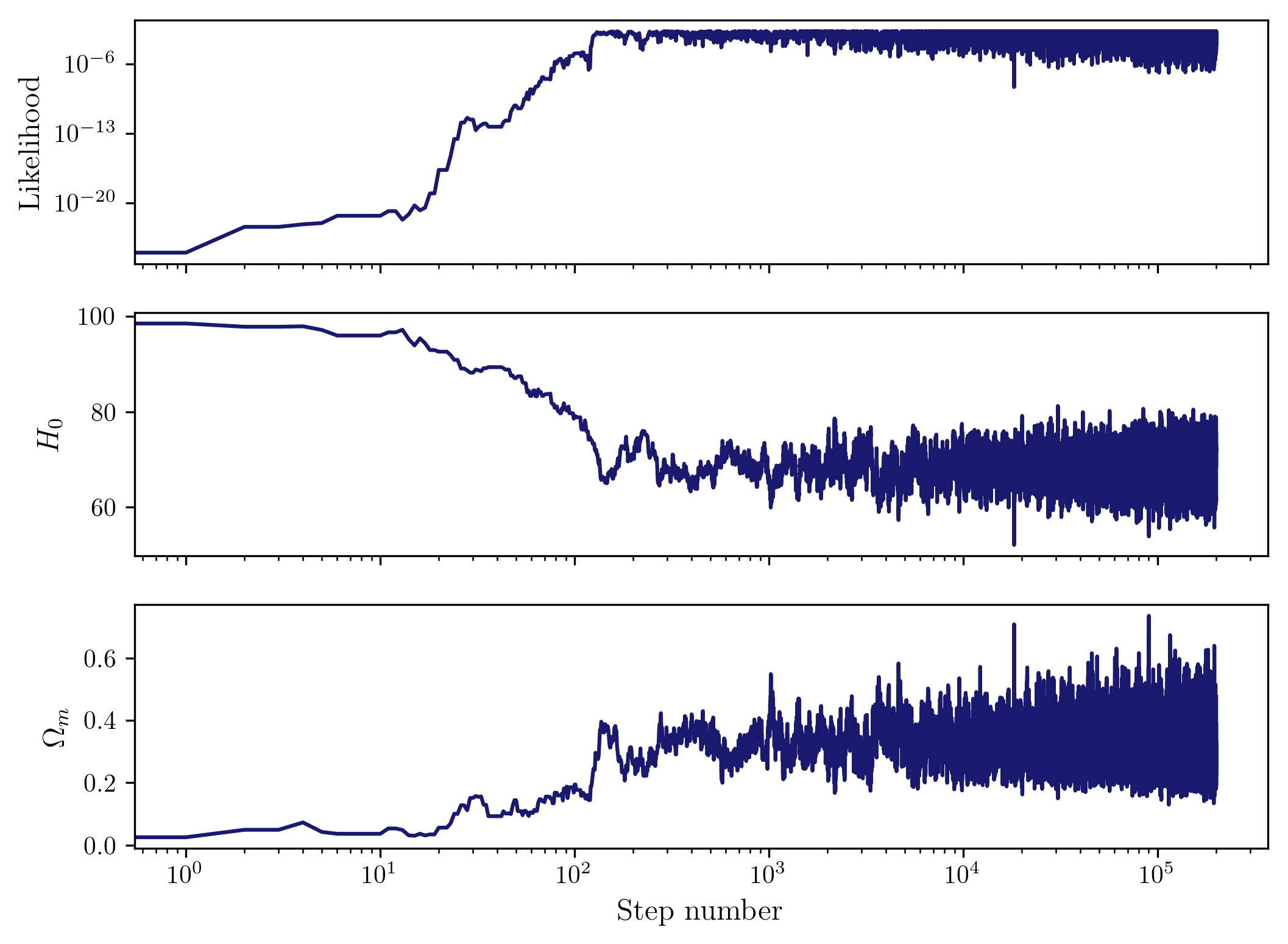
So we see that the chains have converged. We can look at the parameters in a chain as a function of step, and we should see the burn-in phase at the start of the chain, and then the sampling around the preferred values of the parameters and their uncertainties given the data.
# Let's look at the chains.
plt.figure(figsize=(8,5))
plot_params(chain3)
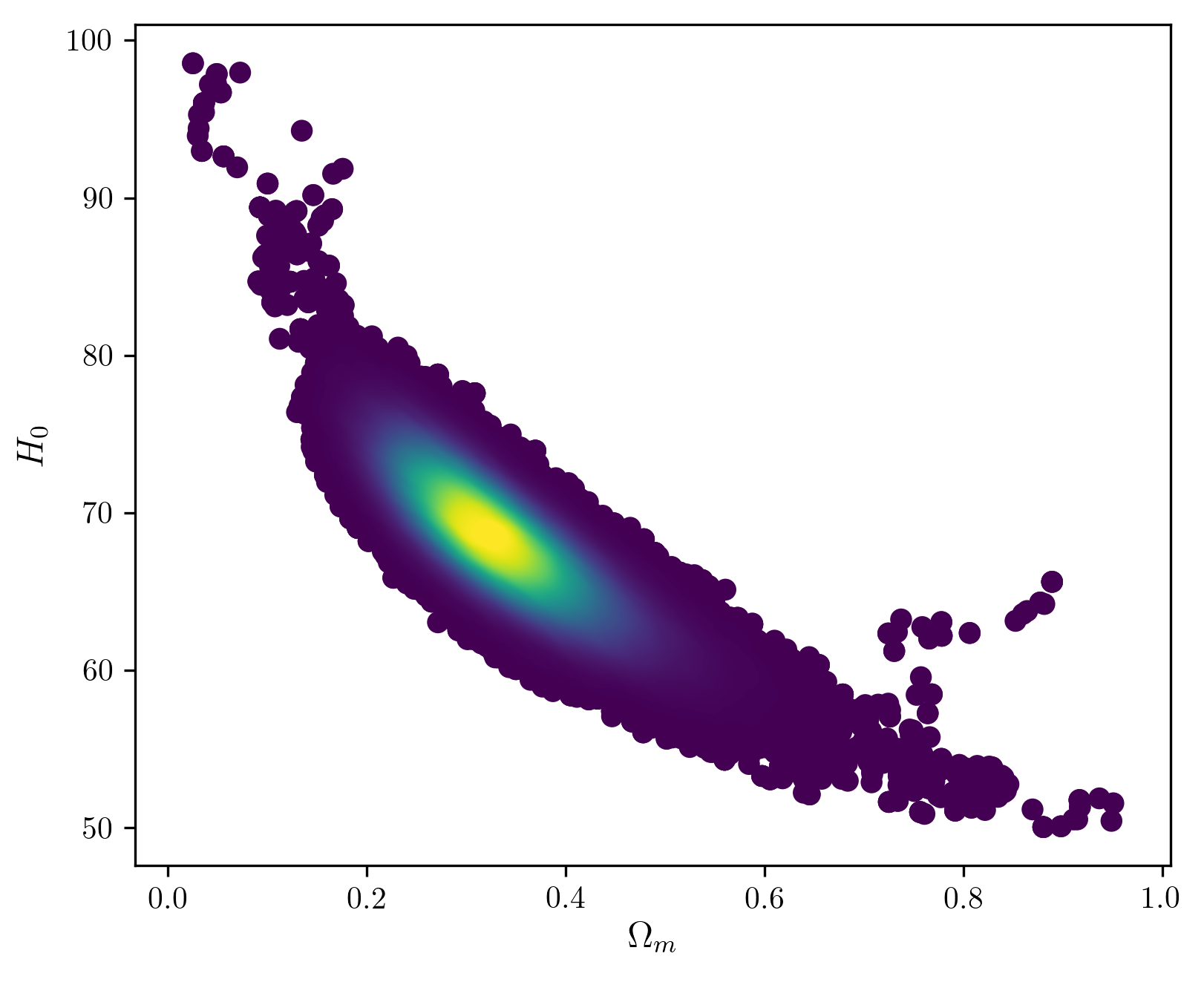
Now we can join the chains and plot the density of points in the 2D parameter space, which gives us the posterior at each point.
# Joining the chains
chains = np.vstack([chain1,chain2,chain3,chain4])
plt.figure(figsize=(8,5))
plot_chain(chains,True)
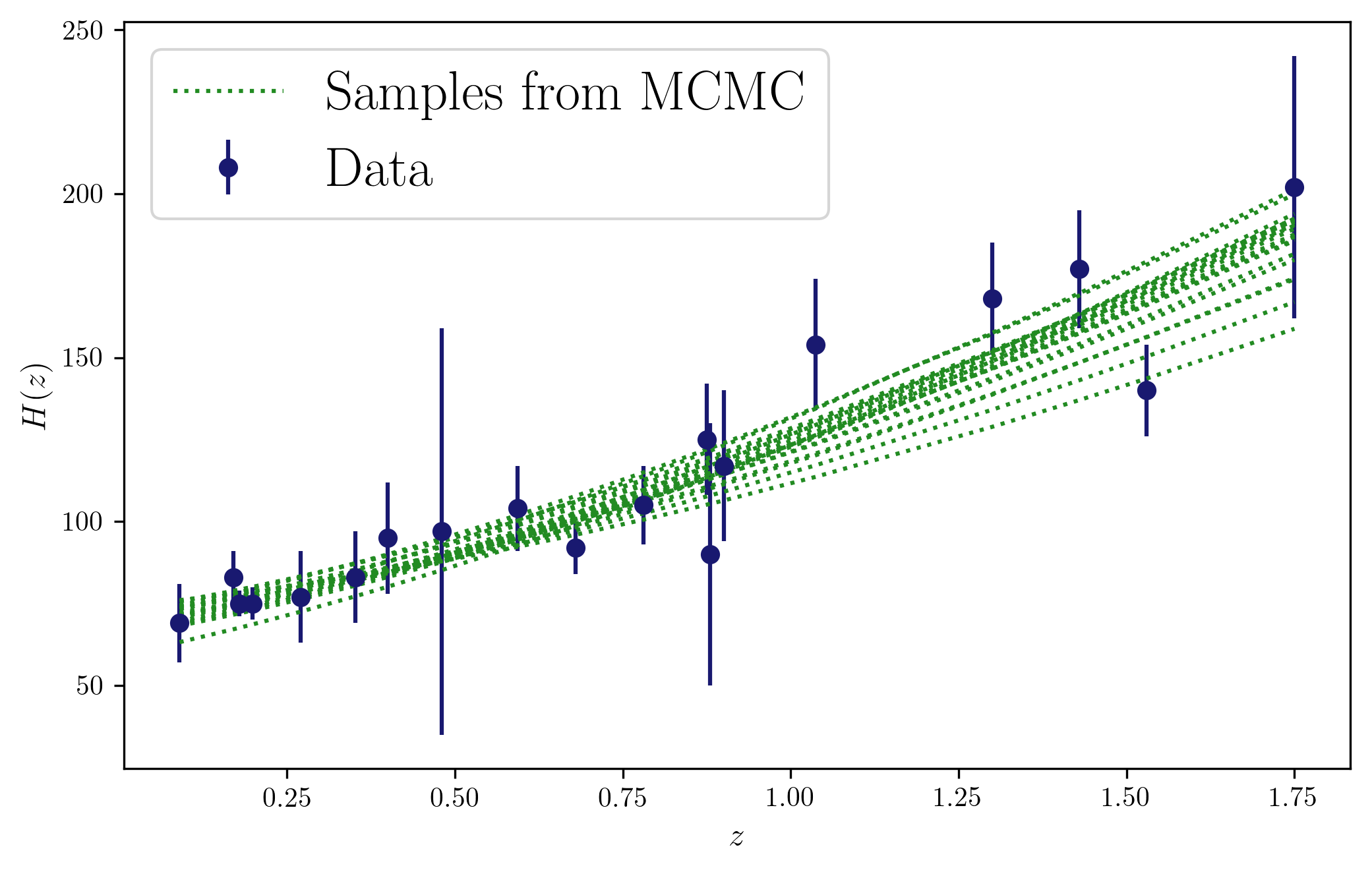
Now we can look at different (random) samples from the chains, and visually check their consistency with the data…
ids = np.random.randint(0,len(chains[:,0]), size=20)
plt.figure(figsize=(8,5))
plt.xlabel(r'$z$',size='large')
plt.ylabel(r'$H(z)$',size='large')
plt.errorbar(z,h,h_err,c='midnightblue',ls='',fmt='o',label='Data')
for id in ids:
    plt.plot(z,hofz(z,chains[id,0],chains[id,1]),c='forestgreen',ls='dotted',label='Samples from MCMC' if id == ids[0] else "")
plt.legend(fancybox=True,fontsize=20,loc=2)
plt.savefig('plot_mcmc_04.png',dpi=300,bbox_inches = 'tight')
Going further…
-
Use informative priors! For instance, from another experiment.
-
We could look at more complicated models, adding parameters to the problem. For instance, for a non-flat universe with a dark energy equation of state parametrized as \(w(z) = w + w_a(1 - a)\), the model would look like this:
-
The MCMC implementation here is most likely not optimal… More sophisticated samplers are available and probably much faster and very easy to use. One popular example in python is emcee, which is also well documented. In order to analyze chains, there are also good codes available online. In DES, we typically use chainconsumer, with which you can produce plots like the one above using just 3 lines of code, and it will take the exact output from emcee.
-
When checking the public MCMC implementations like emcee, you may notice that they mostly work with log likelihoods instead of likelihoods. There are several reasons why this is a more convenient approach, both from the mathematical and computational points of view, so if planning to use MCMC’s for more complicated cases, that is probably the way to go.
I wrote this tutorial for a hands-on exercise on Monte Carlo methods, including undergraduate and graduate students, at the Department of Physics and Astronomy, University of Pennsylvania, in 2019. The real data example I use is based on a tutorial given to me when I was starting my PhD (perhaps around 2015?), by Prof. Licia Verde (one of the authors of the paper that is used).